Examples¶

After installing WfBase you can run the following quick example either as:

python example_quick.py

or by making the script executable:

chmod u+x example_quick.py

and then executing it with:

./example_quick.py

After you have executed the script, in that same folder files fig_quick_latex.png and fig_quick.pdf should appear.

You can download each example script below individually by clicking on the link under each example. Alternatively, you can download all example files as a single zip file

to unzip this file use the following unix command:

unzip all_examples_python.zip

Anomalous Hall conductivity¶

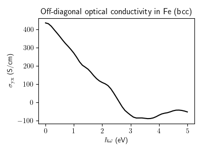
Calculation of an off-diagonal optical conductivity of iron as a function of frequency. Zero frequency limit corresponds to the anomalous Hall conductivity. For demonstration purposes, this calculation uses a rather large smearing eta parameter and a relatively small k-point mesh.

# Copyright under GNU General Public License 2024
# by Sinisa Coh (see gpl-wfbase.txt)

import wfbase as wf
import pylab as plt

wf.download_data_if_needed()

db = wf.load("data/fe_bcc.wf")

# show information about the database file
db.info()

# interpolate quantities to a 16^3 k-mesh
comp = db.do_mesh([16, 16, 16], to_compute = ["A"])

# change the default value of photon energy
comp.compute_photon_energy("hbaromega", 0.0, 5.0, 51)

# change the default value of constant eta
comp["eta"] = 0.3

# this is equation 12.11 for sigma, as written in
# the user_guide.pdf of Wannier90 https://wannier.org/support/
comp.evaluate("sigma_oij <= (j / (numk * volume)) * (f_km - f_kn) * \
               Real((E_km - E_kn) / (E_km - E_kn - hbaromega_o - j*eta)) * \
               A_knmi * A_kmnj")

print("Units of sigma are: ", comp.get_units("sigma"))

# prints to the screen information about quantity sigma evaluated above
comp.info("sigma", show_code = True)

# parse equation into a LaTeX and plot it to a file
wf.render_latex(comp.get_latex("sigma"), "fig_ahc_latex.png")

# the following line will work in iTerm2 and similar terminals
# that support imgcat
wf.display_in_terminal("fig_ahc_latex.png")
# the following line should work in any terminal
#wf.display_in_separate_window("fig_ahc_latex.png")

# compute in SI and multiply with e^2/hbar
result, result_latex = comp.compute_in_SI("sigma", "e^2 / hbar")

# plot latex'ed information about the sigma converted to SI units
#wf.render_latex(result_latex, "fig_ahc_si_latex.png")

fig, ax = plt.subplots(figsize = (4.0, 3.0))
ax.plot(comp["hbaromega"], result[:, 1, 0].real / 100.0, "k-")
ax.set_xlabel(r"$\hbar \omega$ (eV)")
ax.set_ylabel(r"$\sigma_{\rm yx}$ (S/cm)")
ax.set_title("Off-diagonal optical conductivity in Fe (bcc)")
fig.tight_layout()
fig.savefig("fig_ahc.pdf")

Information about the database file¶

This example prints to the screen information about the DFT calculation, and processing, used to generate the database entry stored in file data/au_fcc.wf

See Database for more details.

# Copyright under GNU General Public License 2024
# by Sinisa Coh (see gpl-wfbase.txt)

import wfbase as wf

wf.download_data_if_needed()

db = wf.load("data/au_fcc.wf")

db.info()

Information about the quantities¶

This example prints to the screen information about the quantities stored in the computator object comp, as well as information about the newly computed quantity sigma.

See Quantities for more details.

# Copyright under GNU General Public License 2024
# by Sinisa Coh (see gpl-wfbase.txt)

import wfbase as wf

wf.download_data_if_needed()

# loads the database file
db = wf.load("data/au_fcc.wf")

# creates a computator on a 8x8x8 k-mesh of points
comp = db.do_mesh([8, 8, 8])

# prints information about all quantities currently in comp
comp.info()

# this computes new quantity called "sigma"
comp.evaluate("sigma_oij <= (j / (numk * volume)) * (f_km - f_kn) * \
               Real((E_km - E_kn) / (E_km - E_kn - hbaromega_o - j*eta)) * \
               A_knmi * A_kmnj")

# prints information about newly calculated quantity "sigma"
comp.info("sigma", show_code = True)

Inter- and intra-band optical conductivity¶

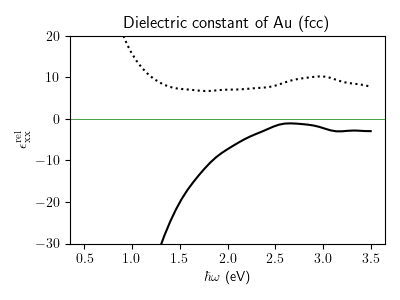
Calculation of inter-band and intra-band optical conductivity of gold, as a function of frequency. For demonstration purposes, we are using here a relatively large smearing of 0.2 eV and a small number of k-points (10^3).

In this example, we use the doublet-notation, so that bands are indexed with pair (n, N) and not a single n index as usual. Therefore index n goes over 9 values, while N goes over 2 values. (Without doublet notation single index n would go over 9*2=18 values.) You can find more details in the description of parameter doublet_indices in the function do_mesh.

Our bands in this example are doubly-degenerate, due to the presence of the combined symmetry of inversion and time-reversal. Therefore, we need to exclude from the inter-band calculation below all terms where (n, N) and (m, M) correspond to the same doublet. In other words, we need to exclude terms for which n is equal to m. This is achieved by the second parameter (conditions) sent to the function evaluate.

# Copyright under GNU General Public License 2024
# by Sinisa Coh (see gpl-wfbase.txt)

import wfbase as wf
import numpy as np
import pylab as plt

wf.download_data_if_needed()

db = wf.load("data/au_fcc.wf")

comp = db.do_mesh([10, 10, 10],
                  shift_k = "random",
                  to_compute = ["A", "dEdk"],
                  doublet_indices = True)

comp.compute_photon_energy("hbaromega", 0.5, 3.5, 51)
comp.compute_hbar_velocity("hbarv")
comp.new("kbtemp", "0.05 * eV")

comp.compute_occupation("f", "E", "ef", "kbtemp")
comp.compute_occupation_derivative("dfdE", "E", "ef", "kbtemp")

comp.replace("eta", "0.2 * eV")

# Chapter 6, Eqs 25 and 26
# https://www.sciencedirect.com/science/article/abs/pii/S1572093406020063
comp.evaluate("""
sigma~intra_oij <= (j / (numk * volume)) * \
    (-dfdE_knN) * (hbarv_knNnNi * hbarv_knNnNj) / (hbaromega_o + j*eta)
sigma~inter_oij <= (j / (numk * volume)) * \
    ((f_kmM - f_knN) * hbarv_knNmMi * hbarv_kmMnNj) /((E_kmM - E_knN) * (E_kmM - E_knN - hbaromega_o - j*eta))
chi_oij <= j * (sigma~intra_oij + sigma~inter_oij) / hbaromega_o
""", "m != n")

wf.render_latex(comp.report(), "fig_sigma_latex.png")

result, result_latex = comp.compute_in_SI("chi", "e^2 / epszero")
wf.render_latex(result_latex, "fig_sigma_chi_latex.png")

eps_xx = 1.0 + result[:,0,0]

fig, ax = plt.subplots(figsize = (4.0, 3.0))
ax.plot(comp["hbaromega"], np.real(eps_xx), "k-")
ax.plot(comp["hbaromega"], np.imag(eps_xx), "k:")
ax.axhline(0.0, c = "g", lw = 0.5)
ax.set_xlabel(r"$\hbar \omega$ (eV)")
ax.set_ylabel(r"$\epsilon^{\rm rel}_{\rm xx}$")
ax.set_title("Dielectric constant of Au (fcc)")
ax.set_ylim(-30, 20)
fig.tight_layout()
fig.savefig("fig_sigma.pdf")

Inter- and intra-band optical conductivity (all metals)¶

The same calculation of inter-band and intra-band optical conductivity, this time done for all transition metals.

Sc (bcc), Ti (bcc), V (bcc), Cr (bcc), Mn (bcc), Fe (bcc), Co (bcc), Ni (bcc), Cu (bcc), Zn (bcc), Y (bcc), Zr (bcc), Nb (bcc), Mo (bcc), Tc (bcc), Ru (bcc), Rh (bcc), Pd (bcc), Ag (bcc), Cd (bcc), Hf (bcc), Ta (bcc), W (bcc), Re (bcc), Os (bcc), Ir (bcc), Pt (bcc), Au (bcc), Hg (bcc)

# Copyright under GNU General Public License 2024
# by Sinisa Coh (see gpl-wfbase.txt)

import wfbase as wf
import numpy as np
import pylab as plt

cases = """sc ti v  cr mn fe co ni cu zn
           y  zr nb mo tc ru rh pd ag cd
           XX hf ta w  re os ir pt au hg"""

wf.download_data_if_needed()

fig, axs = plt.subplots(3, 10, figsize = (20, 6))
row = 0
for line in cases.split("\n"):
    column = 0
    for ll in line.split(" "):
        if ll == "":
            continue
        if ll == "XX":
            axs[row][column].remove()
            column += 1
            continue

        db = wf.load("data/" + ll + "_bcc.wf")

        if ll in ["fe", "co", "ni"]:
            comp = db.do_mesh([10, 10, 10], shift_k = "random", to_compute = ["A", "dEdk"])
        else:
            comp = db.do_mesh([10, 10, 10], shift_k = "random", to_compute = ["A", "dEdk"], doublet_indices = True)
        comp.compute_photon_energy("hbaromega", 0.5, 3.5, 51)
        comp.compute_hbar_velocity("hbarv")
        comp.new("kbtemp", "0.05 * eV")
        comp.compute_occupation("f", "E", "ef", "kbtemp")
        comp.compute_occupation_derivative("dfdE", "E", "ef", "kbtemp")
        comp.replace("eta", "0.2 * eV")
        ev_str = """
        sigma~intra_oij <= (j / (numk * volume)) * (-dfdE_knN) * (hbarv_knNnNi * hbarv_knNnNj) / (hbaromega_o + j*eta)
        sigma~inter_oij <= (j / (numk * volume)) * ((f_kmM - f_knN) * hbarv_knNmMi * hbarv_kmMnNj) /((E_kmM - E_knN) * (E_kmM - E_knN - hbaromega_o - j*eta))
        chi_oij <= j * (sigma~intra_oij + sigma~inter_oij) / hbaromega_o
        """
        if ll in ["fe", "co", "ni"]:
            ev_str = ev_str.replace("M", "").replace("N", "")
        comp.evaluate(ev_str, "m != n")
        result, result_latex = comp.compute_in_SI("chi", "e^2 / epszero")
        eps_xx = 1.0 + result[:,0,0]

        ax = axs[row][column]
        ax.plot(comp["hbaromega"], np.real(eps_xx), "k-")
        ax.plot(comp["hbaromega"], np.imag(eps_xx), "k:")
        ax.axhline(0.0, c = "g", lw = 0.5)
        if row == 2:
            ax.set_xlabel(r"$\hbar \omega$ (eV)")
        if column == 0:
            ax.set_ylabel(r"$\epsilon^{\rm rel}_{\rm xx}$")
        ax.set_ylim(-40, 40)
        ax.set_title(ll.title() + " (bcc)")
        column += 1
    row += 1
fig.tight_layout()
fig.savefig("fig_sigma_all.pdf")

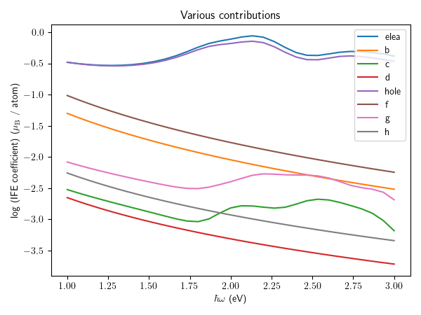
Spin part of inverse Faraday effect¶

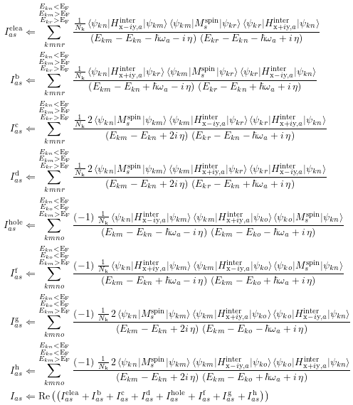
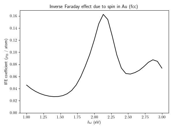
Calculation of the spin part of the inverse Faraday effect. Again, here for demonstration purposes, we are using a rather small k-point sampling and large smearing eta.

More details about the spin part of the inverse Faraday effect can be found in this paper,

https://doi.org/10.1103/PhysRevB.107.214432

# Copyright under GNU General Public License 2024
# by Sinisa Coh (see gpl-wfbase.txt)

import wfbase as wf
import numpy as np
import pylab as plt

wf.download_data_if_needed()

db = wf.load("data/au_fcc.wf")

comp = db.do_mesh([10, 10, 10], to_compute = ["A", "S"])

# increase smearing
comp["eta"] = 0.2

comp.compute_photon_energy("hbaromega", 1.0, 3.0, 31)
comp.compute_optical_offdiagonal_polarization("L", "hbaromega", "x - i y")

comp.evaluate("""
I~elea_as <= (1/numk) *     L_knma *  S_kmrs * #L_knra / ((E_km - E_kn - hbaromega_a -  j*eta)*(E_kr - E_kn - hbaromega_a + j*eta))
I~b_as    <= (1/numk) *    #L_krna *  S_kmrs *  L_krna / ((E_km - E_kn + hbaromega_a -  j*eta)*(E_kr - E_kn + hbaromega_a + j*eta))
I~c_as    <= (1/numk) * 2 * S_knms *  L_kmra * #L_knra / ((E_km - E_kn               + 2j*eta)*(E_kr - E_kn - hbaromega_a + j*eta))
I~d_as    <= (1/numk) * 2 * S_knms * #L_krma *  L_krna / ((E_km - E_kn               + 2j*eta)*(E_kr - E_kn + hbaromega_a + j*eta))
""", "E_kn < ef, E_km > ef, E_kr > ef")

comp.evaluate("""
I~hole_as <= (-1) * (1/numk) *     L_knma * #L_koma *  S_kons / ((E_km - E_kn - hbaromega_a -  j*eta)*(E_km - E_ko - hbaromega_a + j*eta))
I~f_as    <= (-1) * (1/numk) *    #L_kmna *  L_kmoa *  S_kons / ((E_km - E_kn + hbaromega_a -  j*eta)*(E_km - E_ko + hbaromega_a + j*eta))
I~g_as    <= (-1) * (1/numk) * 2 * S_knms * #L_koma *  L_kona / ((E_km - E_kn               + 2j*eta)*(E_km - E_ko - hbaromega_a + j*eta))
I~h_as    <= (-1) * (1/numk) * 2 * S_knms *  L_kmoa * #L_knoa / ((E_km - E_kn               + 2j*eta)*(E_km - E_ko + hbaromega_a + j*eta))
I_as <= Real(I~elea_as + I~b_as + I~c_as + I~d_as + I~hole_as + I~f_as + I~g_as + I~h_as)
""", "E_kn < ef , E_ko < ef, E_km > ef")

wf.render_latex(comp.report(), "fig_ife_latex.png")

print("Units of ife are: ", comp.get_units("I"))

fig, ax = plt.subplots(figsize = (6.0, 4.5))
ax.plot(comp["hbaromega"], comp["I"][:, 2].real, "k-")
ax.set_ylim(0.0)
ax.set_xlabel(r"$\hbar \omega$ (eV)")
ax.set_ylabel("IFE coefficient " + r"($\mu_{\rm B}$ / atom)" )
ax.set_title("Inverse Faraday effect due to spin in Au (fcc)")
fig.tight_layout()
fig.savefig("fig_ife.pdf")

fig, ax = plt.subplots(figsize = (6.0, 4.5))
for x in ["I~elea", "I~b", "I~c", "I~d", "I~hole", "I~f", "I~g", "I~h"]:
    ax.plot(comp["hbaromega"], np.log10(np.abs(comp[x][:, 2].real)), "-", label = x.split("~")[1])
ax.legend()
ax.set_xlabel(r"$\hbar \omega$ (eV)")
ax.set_ylabel("log (IFE coefficient) " + r"($\mu_{\rm B}$ / atom)" )
ax.set_title("Various contributions")
fig.tight_layout()
fig.savefig("fig_ife_contrib.pdf")

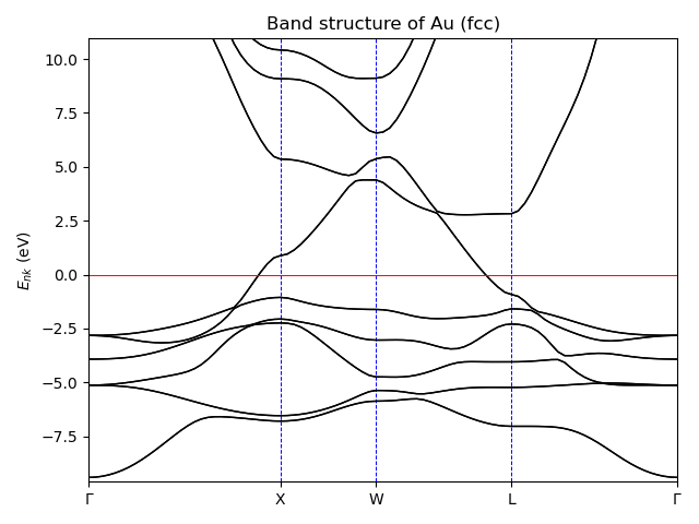
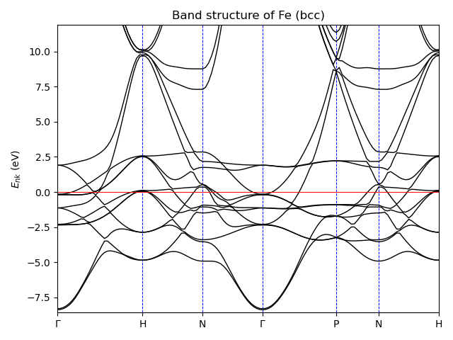
Band structure plot¶

Electron band-structure plot along the high-symmetry lines in the Brillouin zone.

# Copyright under GNU General Public License 2024
# by Sinisa Coh (see gpl-wfbase.txt)

import wfbase as wf
import pylab as plt

wf.download_data_if_needed()

db = wf.load("data/au_fcc.wf")
comp = db.do_path("GM--X--W--L--GM")
fig, ax = plt.subplots()
comp.plot_bs(ax)
ax.set_ylabel(r"$E_{nk}$ (eV)")
ax.set_title("Band structure of Au (fcc)")
fig.tight_layout()
fig.savefig("fig_bs_au.pdf")

db = wf.load("data/fe_bcc.wf")
comp = db.do_path("GM--H--N--GM--P--N--H")
fig, ax = plt.subplots()
comp.plot_bs(ax)
ax.set_title("Band structure of Fe (bcc)")
ax.set_ylabel(r"$E_{nk}$ (eV)")
fig.tight_layout()
fig.savefig("fig_bs_fe.pdf")

Spin-resolved band structure¶

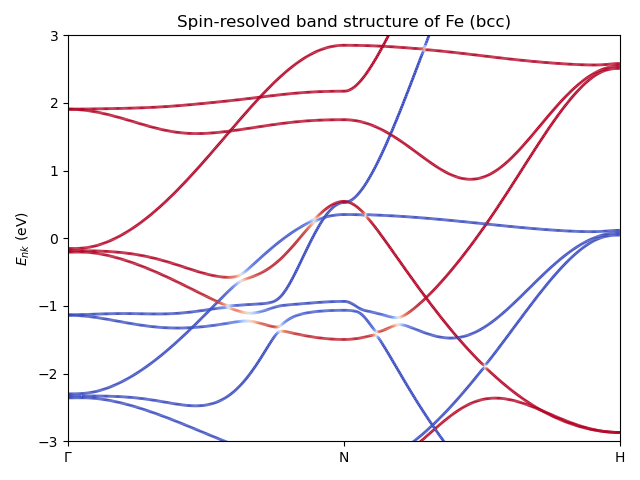
Spin resolved band structure of Fe (bcc) near the Fermi level.

# Copyright under GNU General Public License 2024
# by Sinisa Coh (see gpl-wfbase.txt)

import wfbase as wf
import numpy as np
import pylab as plt

def plot_multicolor_line(ax, x, y, col, rng = None, lw = 2.0, cmap = "coolwarm", negative = True):
    from matplotlib.collections import LineCollection
    points = np.array([x, y]).T.reshape(-1, 1, 2)
    segments = np.concatenate([points[:-1], points[1:]], axis=1)
    if rng is None:
        rng = np.max(np.abs(col))
    if negative == True:
        norm = plt.Normalize(-rng, rng)
    else:
        norm = plt.Normalize(0.0, rng)
    lc = LineCollection(segments, cmap = cmap, norm=norm)
    lc.set_array(col)
    lc.set_linewidth(lw)
    line = ax.add_collection(lc)

wf.download_data_if_needed()

db = wf.load("data/fe_bcc.wf")
comp = db.do_path("GM--N--H", num_steps_first_segment = 300, to_compute = ["S"])
fig, ax = plt.subplots()
comp.plot_bs(ax, plot_bands = False, plot_fermi = False, plot_spec = False)
for i in range(comp["numwann"]):
    plot_multicolor_line(ax, comp["kdist"], comp["E"][:, i], comp["S"][:,i,i,2].real)
ax.set_title("Spin-resolved band structure of Fe (bcc)")
ax.set_ylabel(r"$E_{nk}$ (eV)")
ax.set_ylim(-3, 3)
fig.tight_layout()
fig.savefig("fig_bs_spin.pdf")

Orbital-resolved band structure¶

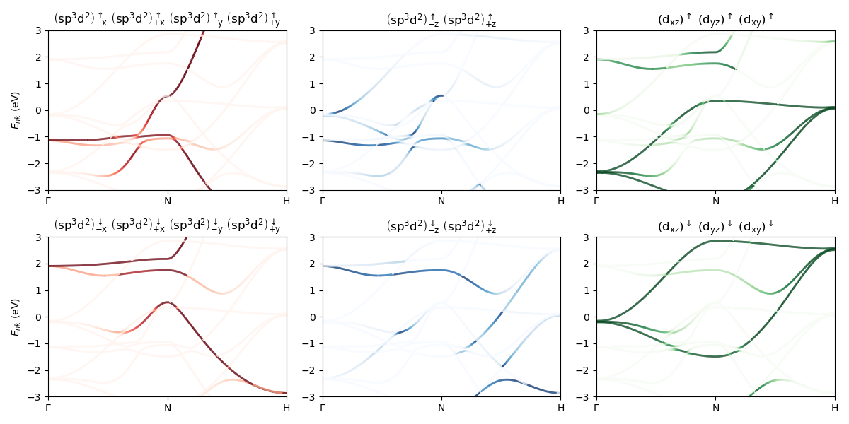
Orbital resolved band structure of Fe (bcc) near the Fermi level.

$\left( {\rm s}{\rm p}^3{\rm d}^2 \right)_{-{\rm x}}^{\uparrow}$ $\left( {\rm s}{\rm p}^3{\rm d}^2 \right)_{+{\rm x}}^{\uparrow}$ $\left( {\rm s}{\rm p}^3{\rm d}^2 \right)_{-{\rm y}}^{\uparrow}$ $\left( {\rm s}{\rm p}^3{\rm d}^2 \right)_{+{\rm y}}^{\uparrow}$, $\left( {\rm s}{\rm p}^3{\rm d}^2 \right)_{-{\rm z}}^{\uparrow}$ $\left( {\rm s}{\rm p}^3{\rm d}^2 \right)_{+{\rm z}}^{\uparrow}$, $\left( {\rm d}_{\rm xz} \right)^{\uparrow}$ $\left( {\rm d}_{\rm yz} \right)^{\uparrow}$ $\left( {\rm d}_{\rm xy} \right)^{\uparrow}$, $\left( {\rm s}{\rm p}^3{\rm d}^2 \right)_{-{\rm x}}^{\downarrow}$ $\left( {\rm s}{\rm p}^3{\rm d}^2 \right)_{+{\rm x}}^{\downarrow}$ $\left( {\rm s}{\rm p}^3{\rm d}^2 \right)_{-{\rm y}}^{\downarrow}$ $\left( {\rm s}{\rm p}^3{\rm d}^2 \right)_{+{\rm y}}^{\downarrow}$, $\left( {\rm s}{\rm p}^3{\rm d}^2 \right)_{-{\rm z}}^{\downarrow}$ $\left( {\rm s}{\rm p}^3{\rm d}^2 \right)_{+{\rm z}}^{\downarrow}$, $\left( {\rm d}_{\rm xz} \right)^{\downarrow}$ $\left( {\rm d}_{\rm yz} \right)^{\downarrow}$ $\left( {\rm d}_{\rm xy} \right)^{\downarrow}$

# Copyright under GNU General Public License 2024
# by Sinisa Coh (see gpl-wfbase.txt)

import wfbase as wf
import numpy as np
import pylab as plt

def plot_multicolor_line(ax, x, y, col, rng = None, lw = 2.0, cmap = "coolwarm", negative = True):
    from matplotlib.collections import LineCollection
    points = np.array([x, y]).T.reshape(-1, 1, 2)
    segments = np.concatenate([points[:-1], points[1:]], axis=1)
    if rng is None:
        rng = np.max(np.abs(col))
    if negative == True:
        norm = plt.Normalize(-rng, rng)
    else:
        norm = plt.Normalize(0.0, rng)
    lc = LineCollection(segments, cmap = cmap, norm=norm)
    lc.set_array(col)
    lc.set_linewidth(lw)
    line = ax.add_collection(lc)

wf.download_data_if_needed()

db = wf.load("data/fe_bcc.wf")
comp = db.do_path("GM--N--H", num_steps_first_segment = 300, to_compute = ["psi"])

fig, axs = plt.subplots(2, 3, figsize = (3*4.0, 2*3.0))
for i in range(2):
    for j in range(3):
        if j == 0:
            # sp3d2_(+-x,+-y)
            orbs = range( 0 + i,  8, 2)
            cmap = "Reds"
        elif j == 1:
            # sp3d2_(+-z)
            orbs = range( 8 + i, 12, 2)
            cmap = "Blues"
        elif j == 2:
            # t2g
            orbs = range(12 + i, 18, 2)
            cmap = "Greens"
        ax = axs[i][j]
        comp.plot_bs(ax, plot_bands = False, plot_fermi = False, plot_spec = False)
        for n in range(comp["numwann"]):
            chars = np.sum((np.abs(comp["psi"][:, n, :])**2)[:, orbs], axis = 1)
            plot_multicolor_line(ax, comp["kdist"], comp["E"][:, n], chars, cmap = cmap, negative = False)
        if j == 0:
            ax.set_ylabel(r"$E_{nk}$ (eV)")
        ax.set_title(" ".join(list(map(lambda s: "$" + s + "$", comp["orbitallabels"][orbs]))))
        ax.set_ylim(-3.0, 3.0)
fig.tight_layout()
fig.savefig("fig_bs_orbital.pdf")

Band structure (all)¶

Band structure of all transition metals (in a bcc structure).

# Copyright under GNU General Public License 2024
# by Sinisa Coh (see gpl-wfbase.txt)

import wfbase as wf
import pylab as plt

wf.download_data_if_needed()

cases = """sc ti v  cr mn fe co ni cu zn
           y  zr nb mo tc ru rh pd ag cd
           XX hf ta w  re os ir pt au hg"""

fig, axs = plt.subplots(3, 10, figsize = (20, 6))
row = 0
for line in cases.split("\n"):
    column = 0
    for ll in line.split(" "):
        if ll == "":
            continue
        if ll == "XX":
            axs[row][column].remove()
            column += 1
            continue
        db = wf.load("data/" + ll + "_bcc.wf")
        comp = db.do_path("GM--H--N")
        ax = axs[row][column]
        comp.plot_bs(ax)
        if column == 0:
            ax.set_ylabel(r"$E_{nk}$ (eV)")
        ax.set_ylim(-12.0, 12.0)
        ax.set_title(ll.title() + " (bcc)")
        column += 1
    row += 1
fig.tight_layout()
fig.savefig("fig_bs_all.pdf")

Anomalous Hall conductivity, orbital¶

Here we computed sigma resolved by orbital decomposition of electron and hole states. This allows us then to compute the contributions of various orbital characters to the sigma.

$$\hbar \omega$ = 0.5 eV, $\hbar \omega$ = 1.0 eV, $\hbar \omega$ = 1.5 eV, $\hbar \omega$ = 2.0 eV$

# Copyright under GNU General Public License 2024
# by Sinisa Coh (see gpl-wfbase.txt)

import wfbase as wf
import numpy as np
import pylab as plt

wf.download_data_if_needed()

db = wf.load("data/fe_bcc.wf")

all_mat = []

for i in range(5):
    comp = db.do_mesh([16, 16, 16], to_compute = ["psi", "A"], shift_k = "random", reorder_orbitals = True)

    comp.compute_orbital_character("O")

    comp.replace("hbaromega", {"value":[0.5, 1.0, 1.5, 2.0], "units":wf.Units(eV = 1)})

    comp["eta"] = 0.3
    comp.new("Ax", comp["A"][:,:,:,0], "A")
    comp.new("Ay", comp["A"][:,:,:,1], "A")

    comp.evaluate("sigma_opr <= (j / (numk * volume)) * (f_km - f_kn) * \
               Real((E_km - E_kn) / (E_km - E_kn - hbaromega_o - j*eta)) * \
               Ax_knm * Ay_kmn * O_knp * O_kmr")

    result, result_latex = comp.compute_in_SI("sigma", "e^2 / hbar")

    result = result.real / 100.0

    all_mat.append(np.real(result))

all_mat = np.mean(np.array(all_mat), axis = 0)

fig, axs = plt.subplots(1, 4, figsize = (4*5.0, 5.2))
for i in range(4):
    mat = all_mat[i]
    orb_lab = list(map(lambda s: "$" + s + "$", comp["orbitallabels"]))

    maxval = np.max(np.abs(mat))
    axs[i].matshow(mat, vmin = -maxval, vmax = maxval, cmap = "seismic")
    axs[i].set_xticks(list(range(mat.shape[0])))
    axs[i].set_xticklabels(orb_lab, rotation = 45)
    axs[i].set_yticks(list(range(mat.shape[1])))
    axs[i].set_yticklabels(orb_lab)
    axs[i].set_aspect("equal")
    axs[i].set_title("$\hbar \omega$ = " + str(comp["hbaromega"][i]) + " eV")

fig.tight_layout()
fig.savefig("fig_ahc_analysis_orbital.pdf")

Anomalous Hall conductivity, energy¶

Here we computed sigma resolved by k-point and pair of band indices (n and m). This allows us then to compute the contributions of various electron-hole pairs to the sigma.

$$\hbar \omega$ = 0.5 eV, $\hbar \omega$ = 1.0 eV, $\hbar \omega$ = 1.5 eV, $\hbar \omega$ = 2.0 eV$

# Copyright under GNU General Public License 2024
# by Sinisa Coh (see gpl-wfbase.txt)

import wfbase as wf
import numpy as np
import pylab as plt

wf.download_data_if_needed()

db = wf.load("data/fe_bcc.wf")

all_x = []
all_y = []
for i in range(10):
    comp = db.do_mesh([16, 16, 16], to_compute = ["A"], shift_k = "random")

    comp.replace("hbaromega", {"value":[0.5, 1.0, 1.5, 2.0], "units":wf.Units(eV = 1)})

    comp["eta"] = 0.3
    comp.new("Ax", comp["A"][:,:,:,0], "A")
    comp.new("Ay", comp["A"][:,:,:,1], "A")

    comp.evaluate("sigma_oknm <= (j / (numk * volume)) * (f_km - f_kn) * \
               Real((E_km - E_kn) / (E_km - E_kn - hbaromega_o - j*eta)) * \
               Ax_knm * Ay_kmn")
    result, result_latex = comp.compute_in_SI("sigma", "e^2 / hbar")
    result = result.real / 100.0

    comp.evaluate("dife_knm <= E_km - E_kn")

    all_x.append(np.real(comp["dife"]))
    all_y.append(np.real(result))

fig, axs = plt.subplots(1, 4, figsize = (4*4.0, 4.0))
for i in range(4):
    ax = axs[i]
    x = np.ravel(np.array(all_x)[:,:,:])
    y = np.ravel(np.array(all_y)[:,i,:,:,:])
    h, hxedg, hyedg = np.histogram2d(x, y, bins = 101, weights = y, range = [[-1.0, 3.0], [-2.5, 2.5]])
    col_range = np.max(np.abs(h))
    ax.pcolormesh(hxedg, hyedg, h.T, vmin = (-1.0)*col_range, vmax = col_range, cmap = "bwr")
    ax.set_xlim(hxedg[0], hxedg[-1])
    ax.set_ylim(hyedg[0], hyedg[-1])
    ax.set_title("$\hbar \omega$ = " + str(comp["hbaromega"][i]) + " eV")
    ax.set_xlabel(r"$E_{km} - E_{kn}$ (eV)")
    if i == 0:
        ax.set_ylabel(r"$\sigma_{\rm xy}$ contribution")
fig.tight_layout()
fig.savefig("fig_ahc_analysis_energy.pdf")

Simple k-mesh convergence¶

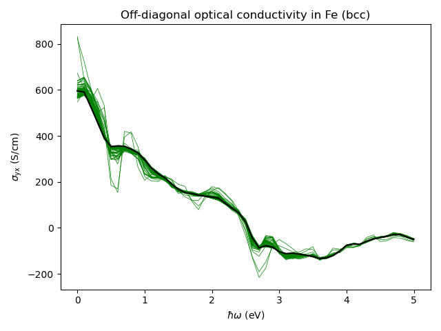
Demonstration of converging calculation with respect to the number of k-points in the mesh. As shown in the previous example, instead of running a single calculation on a large k-mesh (which takes a lot of memory, as all quantities need to be computed on this large k-mesh), the calculation is faster if it is split into many smaller calculations, each with a randomly shifted grid. (If you prefer to do a calculation with a single shot, without splitting it up into smaller randomly shifted grids, then try using evaluate with parameter brute_force_sums set to True. To see how to use this example, take a look at this example.)

The calculation proceeds until the value of optical conductivity does not change too much upon the addition of more k-points.

With the smearing eta set to 0.1 eV, the calculation below needs 71 steps to converge to the relative error of around 0.5 percent. This means that in total one needs 71*8^3 k-points, which is around 36,000 k-points. At smaller smearing one will need to use even more k-points.

While DFT calculations used to create this database are reasonably well-converged, in principle there is no apriori way of knowing whether the physical quantity you are computing is well-converged with respect to these parameters. Therefore, in principle, one would need to check to make sure one has a well-converged calculation with respect to: the energy cut used in the plane-wave DFT calculation used in the creation of the database file data/fe_bcc.wf, smearing parameter, number of k-points in the coarse and fine meshes, frozen and disentanglement windows used in the Wannier90 calculation, structural relaxation, dependence on the exchange-correlation functional, and so on.

However, to change the underlying DFT parameters, you will have to redo the DFT calculations themselves, as these are currently not stored in the database. See the following two examples of how to perform these calculations. First example will show you how to prepare input files for Quantum ESPRESSO and Wannier90. Second example will show you how to perform WfBase calculations once you get output from Quantum ESPRESSO and Wannier90.

Off-diagonal optical conductivity in Fe (bcc)

# Copyright under GNU General Public License 2024
# by Sinisa Coh (see gpl-wfbase.txt)

import wfbase as wf
import numpy as np
import pylab as plt

wf.download_data_if_needed()

db = wf.load("data/fe_bcc.wf")

max_steps = 200

all_values = []
for i in range(max_steps):

    # interpolate quantities to a k-mesh with random shift of k-points
    comp = db.do_mesh([8, 8, 8], shift_k = "random", to_compute = ["A"])

    comp.compute_photon_energy("hbaromega", 0.0, 5.0, 51)
    comp["eta"] = 0.1

    comp.evaluate("sigma_oij <= (j / (numk * volume)) * (f_km - f_kn) * \
                   Real((E_km - E_kn) / (E_km - E_kn - hbaromega_o - j*eta)) * \
                   A_knmi * A_kmnj")

    result, result_latex = comp.compute_in_SI("sigma", "e^2 / hbar")
    all_values.append(result[:, 1, 0].real / 100.0)

    # check if convergence has been achieved
    if len(all_values) > 3:
        res0 = np.mean(all_values[:  ], axis = 0)
        res1 = np.mean(all_values[:-3], axis = 0)
        rdif = np.max(np.abs(res0 - res1))/np.max(np.abs(res0))
        if rdif < 5.0E-3:
            break

    if i == max_steps - 1:
        print("Convergence not achieved in " + str(max_steps) + " steps.")
        exit()

result = np.mean(all_values, axis = 0)

fig, ax = plt.subplots()
ax.plot(comp["hbaromega"], result, "k-", lw = 1.5)
for i in range(len(all_values)):
    average_up_to_i = np.mean(all_values[:i + 1], axis = 0)
    ax.plot(comp["hbaromega"], average_up_to_i, "g-", lw = 0.5, zorder = -1000)
ax.set_xlabel(r"$\hbar \omega$ (eV)")
ax.set_ylabel(r"$\sigma_{\rm yx}$ (S/cm)")
ax.set_title("Off-diagonal optical conductivity in Fe (bcc)")
fig.tight_layout()
fig.savefig("fig_conv.pdf")

Brute-forced sums¶

Compares calculation without brute-forced sums (default, using numpy vectorization) and with brute-forced sums (using Numba). To compare the speed of the two approaches, see the following example.

# Copyright under GNU General Public License 2024
# by Sinisa Coh (see gpl-wfbase.txt)

import wfbase as wf
import numpy as np
import pylab as plt

wf.download_data_if_needed()

db = wf.load("data/fe_bcc.wf")

comp = db.do_mesh([8, 8, 8], shift_k = "random", to_compute = ["A"])
comp.compute_photon_energy("hbaromega", 0.0, 5.0, 51)
comp["eta"] = 0.1

# this calculation uses numpy vectorizations
comp.evaluate("sigma_oij <= (j / (numk * volume)) * (f_km - f_kn) * \
               Real((E_km - E_kn) / (E_km - E_kn - hbaromega_o - j*eta)) * \
               A_knmi * A_kmnj")

# the extra flag at the end of this function call
# ensures that now we use brute force for loops in Numba instead of numpy vectorization
comp.evaluate("alter_oij <= (j / (numk * volume)) * (f_km - f_kn) * \
               Real((E_km - E_kn) / (E_km - E_kn - hbaromega_o - j*eta)) * \
               A_knmi * A_kmnj", brute_force_sums = True)

difference = np.max(np.abs(comp["sigma"] - comp["alter"]))
print("Difference between two approaches is: ", difference)

assert difference < 1.0E-10

Timing¶

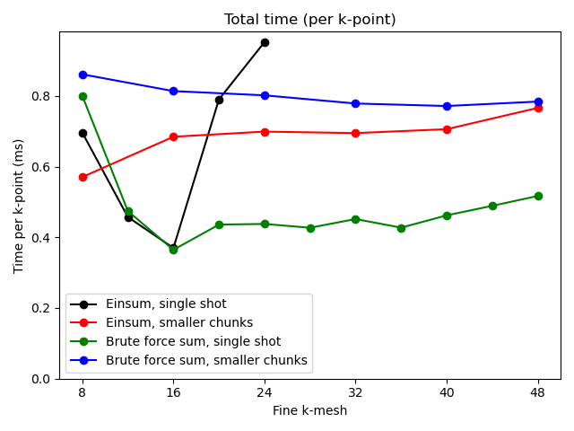
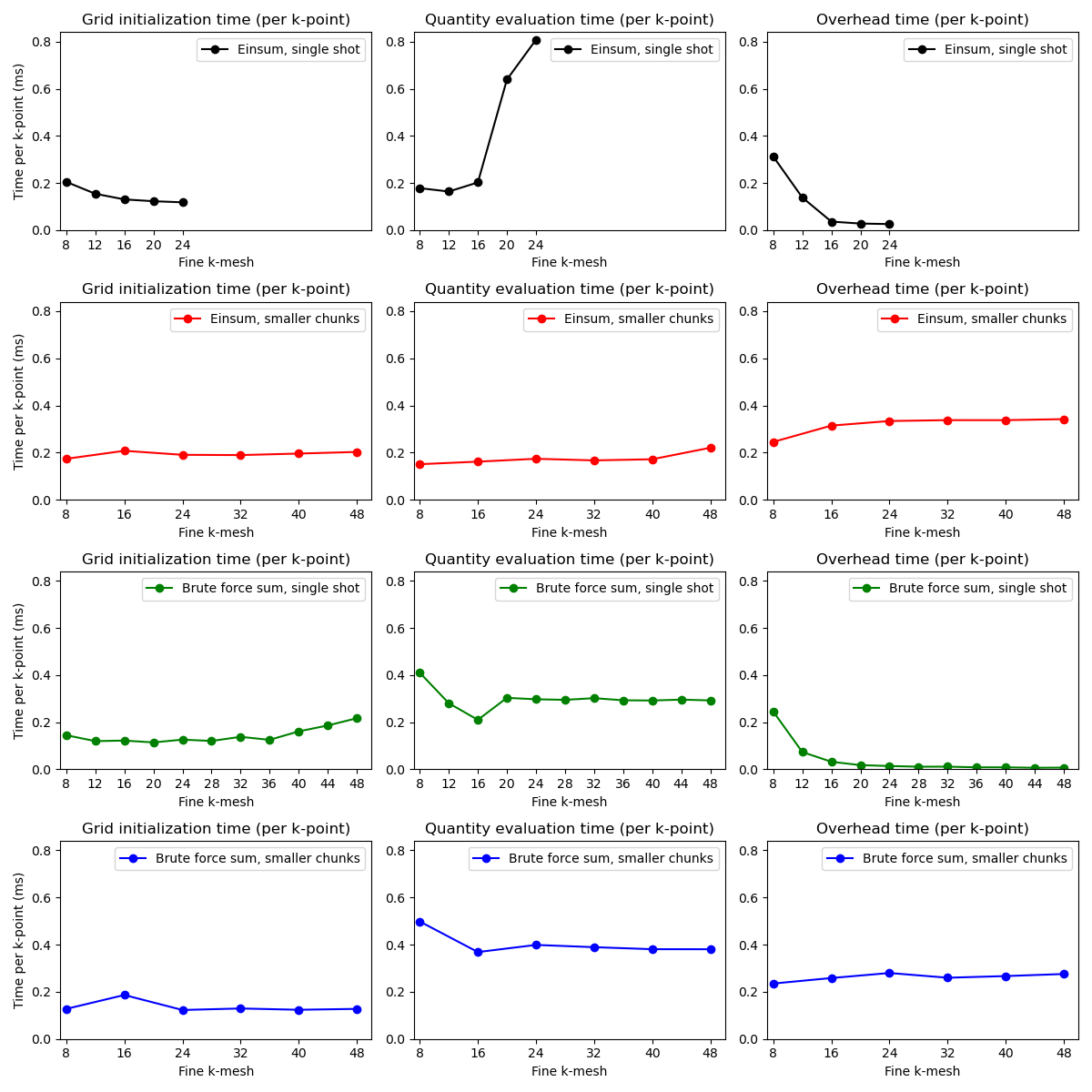
Minimal testing of the speed of computer code is much better than no testing at all. In this simple example, we compare the typical behavior of calculations in wfbase using a computer with 16 GB of RAM. Behavior on your computer might be different.

As the number of k-points in the fine interpolation mesh increases, it becomes less efficient to store all of that information in the memory. Instead, it is more efficient to perform many calculations over smaller grids. This same strategy is used in this example.

On the other hand, if one uses brute forced sums (this uses Numba under the hood) then scaling with a k-point size is better.

These results will also depend on what kind of expression you are using. Depending on the number of distinct indices, and the number of contractions, you might find that brute forced sums (using Numba) might become significantly less efficient than numpy vectorizations.

# Copyright under GNU General Public License 2024
# by Sinisa Coh (see gpl-wfbase.txt)

import wfbase as wf
import numpy as np
import pylab as plt
import time

def main():

    wf.download_data_if_needed()

    db = wf.load("data/fe_bcc.wf")

    figt, axt = plt.subplots()
    fig , axs = plt.subplots(4, 3, figsize = (12.0, 12.0))

    plot_times(check_timings(do_method_1, db, range(8, 25, 4), chunk_size = None), \
               axs[0], axt, "k", "Einsum, single shot")
    plot_times(check_timings(do_method_1, db, range(8, 49, 8), chunk_size = 8   ), \
               axs[1], axt, "r", "Einsum, smaller chunks")
    plot_times(check_timings(do_method_2, db, range(8, 49, 4), chunk_size = None), \
               axs[2], axt, "g", "Brute force sum, single shot")
    plot_times(check_timings(do_method_2, db, range(8, 49, 8), chunk_size = 8   ), \
               axs[3], axt, "b", "Brute force sum, smaller chunks")

    common_axes_range(axs)

    fig.tight_layout()
    fig.savefig("fig_timing.pdf")

    axt.set_ylim(0.0)
    figt.tight_layout()
    figt.savefig("fig_timing_total.pdf")

def do_method_1(db, nk):
    comp = db.do_mesh([nk, nk, nk], shift_k = "random", to_compute = ["A"])
    comp.evaluate("sigma_oij <= (j / (numk * volume)) * (f_km - f_kn) * \
                   Real((E_km - E_kn) / (E_km - E_kn - hbaromega_o - j*eta)) * \
                   A_knmi * A_kmnj")
    return comp

def do_method_2(db, nk):
    comp = db.do_mesh([nk, nk, nk], shift_k = "random", to_compute = ["A"])
    comp.evaluate("sigma_oij <= (j / (numk * volume)) * (f_km - f_kn) * \
                   Real((E_km - E_kn) / (E_km - E_kn - hbaromega_o - j*eta)) * \
                   A_knmi * A_kmnj", brute_force_sums = True)
    return comp

def check_timings(method, db, all_nks, chunk_size = None):

    method(db, 3)

    times = {"nk":[], "tot": [], "ini": [], "exe": []}
    for nk in all_nks:
        print(nk)
        times["nk"].append(nk)
        if chunk_size is None:
            tot_time = time.perf_counter()
            comp = method(db, nk)
            tot_time = time.perf_counter() - tot_time
            times["tot"].append(tot_time)
            times["ini"].append(comp.get_initialization_time())
            times["exe"].append(comp.get("sigma", "total_seconds_exec"))
        else:
            if nk % chunk_size != 0:
                print("Wrong chunk_size.")
                exit()
            nchunks = nk // chunk_size
            tmp_tot_time = 0.0
            tmp_ini_time = 0.0
            tmp_exe_time = 0.0
            for i in range(nchunks**3):
                tot_time = time.perf_counter()
                comp = method(db, chunk_size)
                tot_time = time.perf_counter() - tot_time
                tmp_tot_time += tot_time
                tmp_ini_time += comp.get_initialization_time()
                tmp_exe_time += comp.get("sigma", "total_seconds_exec")
            times["tot"].append(tmp_tot_time)
            times["ini"].append(tmp_ini_time)
            times["exe"].append(tmp_exe_time)
    for k in times.keys():
        times[k] = np.array(times[k])
    return times

def plot_times(times, axs, axt, col, label):
    data_nk  = times["nk"]
    data_tot = 1000.0 * (times["tot"]) / (times["nk"]**3)
    data_ini = 1000.0 * (times["ini"]) / (times["nk"]**3)
    data_exe = 1000.0 * (times["exe"]) / (times["nk"]**3)
    data_ovh = 1000.0 * (times["tot"] - (times["ini"] + times["exe"])) / (times["nk"]**3)

    axt.plot(data_nk, data_tot, col + "o-", label = label)
    axt.set_title("Total time (per k-point)")
    axt.legend()
    axt.set_xticks(data_nk)
    axt.set_xlabel(r"Fine k-mesh")
    axt.set_ylabel(r"Time per k-point (ms)")

    axs[0].plot(data_nk, data_ini, col + "o-", label = label)
    axs[0].set_title("Grid initialization time (per k-point)")
    axs[1].plot(data_nk, data_exe, col + "o-", label = label)
    axs[1].set_title("Quantity evaluation time (per k-point)")
    axs[2].plot(data_nk, data_ovh, col + "o-", label = label)
    axs[2].set_title("Overhead time (per k-point)")
    axs[0].set_ylabel(r"Time per k-point (ms)")
    for ax in axs:
        ax.legend()
        ax.set_xticks(data_nk)
        ax.set_xlabel(r"Fine k-mesh")

def common_axes_range(all_axs):
    xmin = []
    xmax = []
    ymax = []
    for axs in all_axs:
        for ax in axs:
            xmin.append(ax.get_xlim()[0])
            xmax.append(ax.get_xlim()[1])
            ymax.append(ax.get_ylim()[1])
    xmin = max(xmin)
    xmax = max(xmax)
    ymax = max(ymax)
    for axs in all_axs:
        for ax in axs:
            ax.set_xlim(xmin, xmax)
            ax.set_ylim(0.0 , ymax)

main()

Prepare input for DFT calculations¶

This example creates input files for DFT calculations (Quantum ESPRESSO and Wannier90). Script go in the run_dft folder, created by the example script below, gives you information on how to run these DFT calculations.

# Copyright under GNU General Public License 2024
# by Sinisa Coh (see gpl-wfbase.txt)

import wfbase as wf
import pylab as plt

wf.download_data_if_needed()

db = wf.load("data/fe_bcc.wf")

db.create_dft_input_files("run_dft")

print("""You should now take input files in run_dft folder and run
this with your installation of Quantum ESPRESSO and Wannier90. See
script run_dft/go for more details on how to do this.""")

Use the output of DFT calculations¶

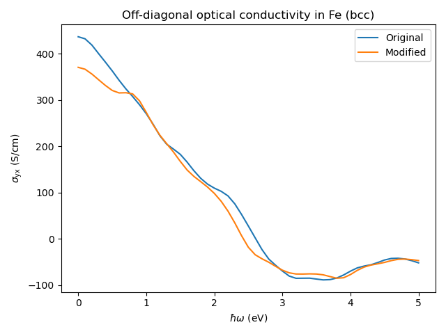
In this example, we use DFT input files prepared in the previous example. We then modified various parameters in those input files and redid the DFT calculations (Quantum ESPRESSO and Wannier90). The example script below reads in the output from Quantum ESPRESSO and Wannier90 and loads those calculations into WfBase.

If you want to redo these calculations on your own, you will need to download the output of the Quantum ESPRESSO and Wannier90 calculations run_dft_output.tar.gz and unpack it in the same folder from which you are running this example script.

The modified calculation below has only 4x4x4 coarse k-mesh (instead of 8x8x8 coarse k-mesh in the original calculation). Furthermore, the modified calculation has fewer empty states.

The modified and original results are quite different, which demonstrates the importance of using dense enough k-meshes in the DFT calculations (and/or enough empty states).

# Copyright under GNU General Public License 2024
# by Sinisa Coh (see gpl-wfbase.txt)

import wfbase as wf
import pylab as plt
import wannierberri as wberri

def main():

    wf.download_data_if_needed()

    fig, ax = plt.subplots()
    for s in range(2):
        if s == 0:
            # regular calulation from wfbase database
            db = wf.load("data/fe_bcc.wf")
            label = "Original"
        elif s == 1:
            # reads in output of DFT calculations using WannierBerri
            # The following line uses WannierBerri syntax.  See here for
            # more details on how to use WannierBerri https://wannier-berri.org
            system = wberri.System_w90("run_dft_output/x", berry = True, spin = False)
            db = wf.load_from_wannierberri(system, global_fermi_level_ev = 18.3776)
            label = "Modified"

        comp = db.do_mesh([16, 16, 16], to_compute = ["A"])
        comp.compute_photon_energy("hbaromega", 0.0, 5.0, 51)
        comp["eta"] = 0.3
        comp.evaluate("sigma_oij <= (j / (numk * volume)) * (f_km - f_kn) * \
        Real((E_km - E_kn) / (E_km - E_kn - hbaromega_o - j*eta)) * \
        A_knmi * A_kmnj")
        result, result_latex = comp.compute_in_SI("sigma", "e^2 / hbar")

        ax.plot(comp["hbaromega"], result[:, 1, 0].real / 100.0, "-", label = label)

    ax.legend()
    ax.set_xlabel(r"$\hbar \omega$ (eV)")
    ax.set_ylabel(r"$\sigma_{\rm yx}$ (S/cm)")
    ax.set_title("Off-diagonal optical conductivity in Fe (bcc)")
    fig.tight_layout()
    fig.savefig("fig_standalone_recalculate.pdf")

if __name__ == "__main__":
    main()

Alternative, equivalent, calculation (only using numpy routines)¶

All quantities in WfBase are simply numpy arrays, and one can directly do the computation with the numpy arrays, without having to use the evaluate routine from WfBase. This approach is demonstrated in the example below. The approach from WfBase is more compact and easier to debug and analyze.

# Copyright under GNU General Public License 2024
# by Sinisa Coh (see gpl-wfbase.txt)

import wfbase as wf
import numpy as np
import pylab as plt
from opt_einsum import contract as opteinsum

wf.download_data_if_needed()

db = wf.load("data/fe_bcc.wf")
comp = db.do_mesh([16, 16, 16], to_compute = ["A"])

# computation using wfbase's evaluate function
comp.evaluate("sigma_oij <= (j / (numk * volume)) * (f_km - f_kn) * \
               Real((E_km - E_kn) / (E_km - E_kn - hbaromega_o - j*eta)) * \
               A_knmi * A_kmnj")

# the user can achieve the same thing by directly
# accessing quantities and using standard numpy operations.
#
# these are simply numpy arrays...
f = comp["f"]
E = comp["E"]
ho = comp["hbaromega"]
A = comp["A"]
# and now we can build up the same expression as above
dif_f = f[:, :, None] - f[:, None, :]
dif_E = E[:, :, None] - E[:, None, :]
dif_E_denom = dif_E[None, :, :, :] - ho[:, None, None, None] - 1.0j * comp["eta"]
fraction = np.real(dif_E[None, :, :, :] / dif_E_denom[:, :, :, :])
sigma = opteinsum("kmn, okmn, knmi, kmnj -> oij", dif_f, fraction, A, A)
sigma = sigma * 1.0j / (comp["numk"] * comp["volume"])

difference = np.max(np.abs(comp["sigma"] - sigma))
print("Difference between two approaches is: ", difference)

assert difference < 1.0E-10

Alternative, equivalent, calculation (WfBase and numpy routines)¶

Calculation of the quantity by directly using both regular numpy routines and WfBase.

# Copyright under GNU General Public License 2024
# by Sinisa Coh (see gpl-wfbase.txt)

import wfbase as wf
import numpy as np
import pylab as plt
from opt_einsum import contract as opteinsum

wf.download_data_if_needed()

db = wf.load("data/fe_bcc.wf")
comp = db.do_mesh([16, 16, 16], to_compute = ["A"])

# computation using wfbase's evaluate function
comp.evaluate("sigma_oij <= (j / (numk * volume)) * (f_km - f_kn) * \
               Real((E_km - E_kn) / (E_km - E_kn - hbaromega_o - j*eta)) * \
               A_knmi * A_kmnj")

# user could instead perform a part of the calculation using regular numpy arrays
# and then add those to the computator above and then run wfbase evaluate.
# As a demonstration, let us compute one of the intermediate objects from
# the equation above:
f = comp["f"]
deltaf = f[:, :, None] - f[:, None, :]
# now we can put this variable back into the computator
comp.new("deltaf", deltaf)
# and now we can use this new quantity in the computation below
comp.evaluate("alternative_oij <= (j / (numk * volume)) * deltaf_kmn * \
               Real((E_km - E_kn) / (E_km - E_kn - hbaromega_o - j*eta)) * \
               A_knmi * A_kmnj")

difference = np.max(np.abs(comp["sigma"] - comp["alternative"]))
print("Difference between two approaches is: ", difference)

assert difference < 1.0E-10

Alternative, equivalent, calculation (only using numpy routines)¶

WfBase under the hood dynamically constructs a numpy python code based on your input to the evaluate(…) function call. You can access this numpy python code directly, and even run it on your own, modify it if you want, and so on.

The example below shows you how to access this numpy python code and how to run it.

# Copyright under GNU General Public License 2024
# by Sinisa Coh (see gpl-wfbase.txt)

import wfbase as wf
import numpy as np
import pylab as plt
from opt_einsum import contract as opteinsum

wf.download_data_if_needed()

db = wf.load("data/fe_bcc.wf")
comp = db.do_mesh([16, 16, 16], to_compute = ["A"])

# computation using wfbase's evaluate function
comp.evaluate("sigma_oij <= (j / (numk * volume)) * (f_km - f_kn) * \
               Real((E_km - E_kn) / (E_km - E_kn - hbaromega_o - j*eta)) * \
               A_knmi * A_kmnj")

# the following line will display the dynamically generated
# numpy python code used to evaluate the expression above
comp.info("sigma", show_code = True)

# the output of the info command above is given
# by the function evaluate_directly below
def evaluate_directly(__object):
    import numpy as np
    from opt_einsum import contract as opteinsum

    _orig_shp = {}
    _f = []
    _s = {}
    __brod00 = np.copy(__object["f"])
    __brod00 = __brod00[:,:,None] - (__object["f"])[:,None,:]
    __brod01 = np.copy(__object["E"])
    __brod01 = __brod01[:,:,None] - (__object["E"])[:,None,:]
    __brod02 = np.array(complex(1.0j))
    __brod02 = __brod02 * (__object["eta"])
    __brod03 = np.copy(__object["E"])
    __brod03 = __brod03[:,:,None,None] - (__object["E"])[:,None,:,None]
    __brod03 = __brod03.squeeze(axis = (3,))
    __brod03 = __brod03[:,:,:,None] - (__object["hbaromega"])[None,None,None,:]
    __brod03 = __brod03 - (__brod02)
    __brod04 = np.copy(__brod01)
    __brod04 = __brod04[:,:,:,None] * ((1.0/(__brod03)))[:,:,:,:]
    __mult00 = opteinsum(",,,kmn,kmno,knmi,kmnj->oij",\
                         complex(1.0j),\
                         (1.0/(__object["numk"])),\
                         (1.0/(__object["volume"])),\
                         __brod00,\
                         np.real(__brod04),\
                         __object["A"],\
                         __object["A"])
    __value = __mult00
    return __value

# now call the function we got printed using info
sigma_alt = evaluate_directly(comp)

difference = np.max(np.abs(comp["sigma"] - sigma_alt))
print("Difference between two approaches is: ", difference)

assert difference < 1.0E-10

Alternative, equivalent, calculation (brute-forced sums using numba)¶

When you call evaluate and set parameter brute_force_sums to True, then WfBase under the hood will dynamically construct a Numba (not numpy) python code based on your input to the evaluate(…) function call. You can access this Numba python code directly, and even run it on your own, modify it if you want, and so on.

The example below shows you how to access this Numba python code and how to run it.

# Copyright under GNU General Public License 2024
# by Sinisa Coh (see gpl-wfbase.txt)

import wfbase as wf
import numpy as np
import pylab as plt
from opt_einsum import contract as opteinsum

wf.download_data_if_needed()

db = wf.load("data/fe_bcc.wf")
comp = db.do_mesh([16, 16, 16], to_compute = ["A"])

# computation using wfbase's evaluate function
comp.evaluate("sigma_oij <= (j / (numk * volume)) * (f_km - f_kn) * \
               Real((E_km - E_kn) / (E_km - E_kn - hbaromega_o - j*eta)) * \
               A_knmi * A_kmnj", brute_force_sums = True)

# the following line will display the dynamically generated
# Numba python code used to evaluate the expression above
comp.info("sigma", show_code = True)

# the output of the info command above is given
# by the function evaluate_directly below
def evaluate_directly(__object):
    from numba import njit
    import numpy as np

    __object_numk = __object["numk"]
    __object_volume = __object["volume"]
    __object_f = __object["f"]
    __size_k = __object.get_shape("f")[0]
    __size_m = __object.get_shape("f")[1]
    __size_n = __object.get_shape("f")[1]
    __object_E = __object["E"]
    __object_hbaromega = __object["hbaromega"]
    __size_o = __object.get_shape("hbaromega")[0]
    __object_eta = __object["eta"]
    __object_A = __object["A"]
    __size_i = __object.get_shape("A")[3]
    __size_j = __object.get_shape("A")[3]

    @njit
    def _tmp_func__000(__value):
        for k in range(__size_k):
            for n in range(__size_n):
                for m in range(__size_m):
                    for o in range(__size_o):
                        for i in range(__size_i):
                            for j in range(__size_j):
                                __value[o,i,j] += (((1.0j) / (__object_numk * __object_volume)) * (__object_f[k,m] - \
                                                  __object_f[k,n]) * (((__object_E[k,m] - __object_E[k,n]) / (__object_E[k,m] - \
                                                  __object_E[k,n] - __object_hbaromega[o] - ((1.0j) * __object_eta)))).real * \
                                                  __object_A[k,n,m,i] * __object_A[k,m,n,j])
    __value = np.zeros((__size_o,__size_i,__size_j), dtype = complex)
    _tmp_func__000(__value)
    return __value

# now call the function we got printed using info
sigma_alt = evaluate_directly(comp)

difference = np.max(np.abs(comp["sigma"] - sigma_alt))
print("Difference between two approaches is: ", difference)

assert difference < 1.0E-10